Published with minor revisions as "Refining Ratings" in the August 1998 issue of Risk.  All figures appear at the end of the article.

A Nonparametric Test for Credit Rating Refinements

by

Ross M. Miller
Miller Risk Advisors
2255 Algonquin Road
Niskayuna, NY 12309 USA

millerrm@alumni.caltech.edu

May 1998

While the intensive quantification of market risk has led to measurements accurate to the basis point (and beyond), difficulties in quantifying credit risk have resulted in the practice of measuring this risk with far less precision. Indeed, financial institutions that develop their own internal measures of credit risk usually employ a "1" to "9" scale of creditworthiness for their exposures, taking their lead from the rating agencies and their AAA to D (and similar) systems. Even with the further refinement of "notches," designated with a "+" or "-" the vast universe of credit risk is reduced to at most thirty buckets. In reality, the broad range of pricing for corporate debt obligations in the marketplace indicates that there are far more than thirty categories of credit risk. In the high-yield debt market the illusion of "stability" provided by a broad categorization scheme can be easily outweighed by its imprecision.

The difference in the precision with which market risk and credit risk have been measured is due in large part to the rich body of quantitative theory that has been developed for analyzing market risk. In particular, there are many cases where the arbitrage-based techniques of option valuation theory can be applied to market risk. Despite the numerous shortcomings of this theory (elaborated upon in this and other journals), its practical application leads to a fairly precise quantification of risk in a wide variety of settings.

Fortunately, those same option-theoretic roots that have been so useful in quantifying market risk can be applied to the quantification of credit risk in corporate settings. Indeed, the modern theory’s developers—Fischer Black, Myron Scholes, and Robert Merton—noted in their earliest work on options that the equity in any firm could itself be valued as an option. The value of the equityholder’s implicit option is directly related to the likelihood of financial distress, at which point they will choose to limit any further liability from their stake in the firm by "putting" it at a price of zero to the debtholders. Generally, such financial distress will also result in a shortfall to the debtholders and the firm will default on its debt. Hence, the credit risk of the firm, i.e., its propensity to default, is directly and quantitatively linked to the value of its equity. In those cases where the value of the equity is directly observable, such as when it takes the form of an actively-traded security, one should be able, in principle, to "reverse engineer" the probability distribution of default from the market value of the equity given the volatility and financial structure of the firm’s assets. Without delving into the messy details here, the option-valuation approach to credit risk is far more difficult to make practical than its market risk analogue.

This paper develops and applies the statistical machinery that is necessary to determine whether a particular quantitative method of measuring credit risk, using option valuation or other methods, truly represents a refinement over broader categorization methods. Here the term "refinement" is used in a technical sense of partitioning the creditworthiness of firms in a way that yields more information that the original partition, in this case the letter-based ratings. This is a particularly challenging statistical problem because defaults themselves are infrequent occurrences and the error structure of their estimates cannot be assumed to be normal or any other well-behaved distribution. The solution to this problem is to get the most out of the data that exists and to apply nonparametric tests, which do not rely on distributional assumptions, to these data. Although this paper applies the methodology to a specific refinement of letter-based ratings, it can be applied quite broadly.

Alternative Credit Ratings

The methodology for testing whether a quantitative credit rating system is a statistically significant refinement of a broader rating system that is described here was developed as part of an independent study commissioned by the Capital Markets Assurance Corporation (CapMAC), a financial guarantee company based in New York that subsequently merged with MBIA Inc., another financial guarantee company. Specifically, CapMAC was interested in the degree to which the quantitative credit ratings provided by KMV Corporation’s Credit Monitor system, the first option-based credit rating system, were a refinement of Standard & Poor’s (S&P) notch-level ratings for U.S. companies.

For this study S&P’s senior unsecured debt ratings as they appear in Compustat were used. The S&P company ratings that were used were (in descending order of credit quality): AAA, AA+, AA, AA-, A+, A, A-, BBB+, BBB, BBB-, BB+, BB, BB-, B+, B, B-. Ratings below B- (CCC+, CCC, etc.) were excluded from the study because of the sparseness of these data. S&P ratings are designed to provide intermediate to long-run indications of creditworthiness.

In contrast, KMV’s ratings take the form of expected default frequencies (EDFs), which range from 0.02% (2 basis points) to 20% and are reported with basis point precision, making for 1,999 different possible ratings. Because the likelihood of default varies over the business cycle, there is no fixed mapping between KMV and S&P ratings. KMV provides EDFs for horizons ranging from one to five years (see Kealhofer, Kwok, and Weng, 1998 for more information about Credit Monitor and the relationship between EDFs and agency ratings). For this study, the one-year EDF, for which KMV provides the most information, is used. Although the EDF provides a cardinal measure of credit risk, the nonparametric methods used in this study will only examine its ordinal properties relative to S&P ratings.

The test of KMV’s predictive power relative to an S&P rating can be expressed as the following null hypothesis: given an S&P rating for a company, the KMV rating (EDF) provides no additional information as to the likelihood the firm will default over a specified period of time. Figure 1 gives a grid of the EDFs for all companies rated by KMV Credit Monitor at the end of 1989 that had an S&P company rating of B- in ascending order of EDF (descending creditworthiness). The null hypothesis states that the pattern of defaults should be random within that cohort; however, it is clear from Figure 1 that over the next three years (1990-1992) defaults came disproportionately from the companies with the highest EDFs. Of course, this is a single cohort at a single point in time. In the following section we will demonstrate how to aggregate all cohorts at all points in time into a single nonparametric statistical test of the null hypothesis.

Aggregating Defaults

The study covered U.S. companies on an end-of-month basis from June 1986 to November 1996. Only U.S. companies with both S&P ratings and KMV Credit Monitor EDFs were used—a total of over 1,000 companies at some point during the 10-year sample period. Defaults were taken from KMV’s default database, includes both the defaults reported by the rating agencies for rated issues as well as defaults for companies having no rated debt. Although KMV performed a major revision of its model in 1994, only the EDFs contemporaneously reported by KMV were used in order to minimize the extent to which we were testing the model on data to which it had been backtested or backfitted.

The trick to aggregating the KMV data over both time and S&P ratings categories is to convert each EDF into an ordinal ranking within its month and (notch) rating cohort. A natural ordinal measure is a percentile rank—with 100 being the best (lowest EDF) and 0 the worst (highest EDF). A means for computing percentile that both takes account of ties in ranking, which are quite rare for companies with higher EDFs, and is consistent across cohorts of different sizes is given by:

where Total is the size of the cohort, Worse is the number of the firms in the cohort with worse credit ratings (EDFs), and Better is the number of firms with better ratings.

For example, in a cohort with 20 companies (the smallest allowed in the study), the company with the lowest EDF (assuming it is the only one) has Better = 0, Worse = 19, so by substitution above its Percentile = 97.5 (the midpoint of the top 5%). If two companies are tied for 3^rd and 4^th best EDFs, they would have Better = 2, Worse = 16, giving Percentile = 85.

The reason for a lower limit on the size of a cohort is to make the distribution of percentiles as continuous as possible, facilitating meaningful comparisons between cohorts. Also note that by converting an EDF to a percentile we are completely eliminating any bias that might result from EDFs as a whole being more or less optimistic about the overall rate of defaults than S&P ratings.

The null hypothesis that EDFs provide no information beyond that contained in S&P ratings can be made operational using EDF percentiles. Given the way that the percentiles were constructed, the null hypothesis implies that the percentiles of the population of defaulting firms will have a flat (or uniform) distribution. In particular, looking at defaulting firms any fixed number of months prior to the default, the distribution of percentiles should be uniform.

The histograms in Figure 2 show that at 6 months prior to default this distribution is obviously far from uniform. As time to default increases, the distribution becomes more uniform, which is what one would expect for any system with predictive power, i.e., as the time to the event increases, the predictive power decreases. Nonetheless, just from looking at the graph of the distribution, it is apparent that there is still some predictive power 36 months prior to default.

Applying Kolmogorov-Smirnov

The Kolmogorov-Smirnov test is used to quantify the degree to which the observed distribution differs from uniformity as a statistical significance level. This test is a basic and well-understood tool of nonparametric statistics (see Siegel and Castellan, 1988 for details). In the one-sample version of this test we can determine the significance with which a sample of data differs from a given baseline frequency distribution—in this case the uniform distribution.

The Kolmogorov-Smirnov test works on the distributional characteristics of the maximum distance between the cumulative density functions of the sample and the baseline. This maximum distance is known as the D-statistic. By aggregating over all months and ratings we get at least fifty data points for which both KMV and S&P ratings are known 6, 12, 18, 24, 36 and 48 months prior to default, more than enough to perform a meaningful statistical test.

The results of this test are given in the table below. KMV Credit Monitor has very strong predictive value for as many as 18 months prior to default. The predictive power remains statistically significant out to 36 months. At 48 months the significance level finally drops below 95%.

An alternative nonparametric approach to showing predictive power of EDFs relative to S&P ratings is to apply a binomial test to a division of the sample into two parts, with the 50^th percentile as a natural cutoff point. The results of this test, which are not given here, as well as for other natural percentile cutoffs (90^th, 75^th, etc.) confirm the results of the Kolmogorov-Smirnov test. The advantage of the Kolmogorov-Smirnov test is that it does not require the arbitrary choice of a percentile cutoff.

Discussion

This paper has demonstrated a statistical methodology for inferring that a quantitative credit rating system is a refinement of a traditional rating system, i.e., it provides additional information. This demonstration was made with the use of a single, innocuous statistical assumption—that the number of firms in a cohort is large enough to make the distribution of percentiles nearly continuous. Generating results beyond those given here almost always comes at the cost of additional assumptions that could affect the validity of the analysis. For example, it is natural to try to turn the analysis around and ask whether for a given EDF a letter rating provides additional information. To do this analysis the technique developed above cannot be applied without making further assumptions. The problem here is that while each letter rating-based cohort has associated with it a near-continuum of EDFs (cf. Figure 1), virtually all cohorts based on a single EDF will contain few, if any, companies because the number of companies is small relative to the number of possible EDFs. The remedy of grouping EDFs together to get around this problem not only will require the use of arbitrary cutoffs, but also will throw away information that may then be incorrectly attributed to the letter rating.

Additional assumptions are also required to gauge the relative contribution of both the letter-based and quantitative rating systems simultaneously using regression analysis. In a regression the two rating systems are used to generate two or more dependent variables. The independent variable is then either the default rate (for grouped data) or a dummy variable representing default (for individual data). Whichever way the analysis is set up, explicit assumptions as to the error distribution of the independent variables must be made in order to perform the regression. Given that neither rating is generated by a "natural" process that can be expected to have a predictable error term, e.g., normally distributed, the results are likely to be quite sensitive to the distributional assumptions that underlie the regression.

On a more positive note, the analysis performed in this paper can be readily extended to compare two different quantitative credit rating systems to a common letter-based baseline. Such a comparison can be directly implemented using the two-sample version of the Kolmogorov-Smirnov test, a standard textbook extension of the single-sample version that we used.

References

Kealhofer S, S Kwok and W Weng, 1998
Uses and abuses of bond default rates
CreditMetrics Monitor, First Quarter, pages 37-55

Siegel, S and N. J. Castellan Jr., 1988
Nonparametric statistics for the behavioral sciences, second edition
McGraw-Hill

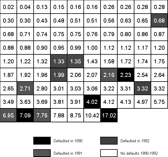
Figure 1. Defaults for S&P B- Companies at the end of 1989 ordered by EDF

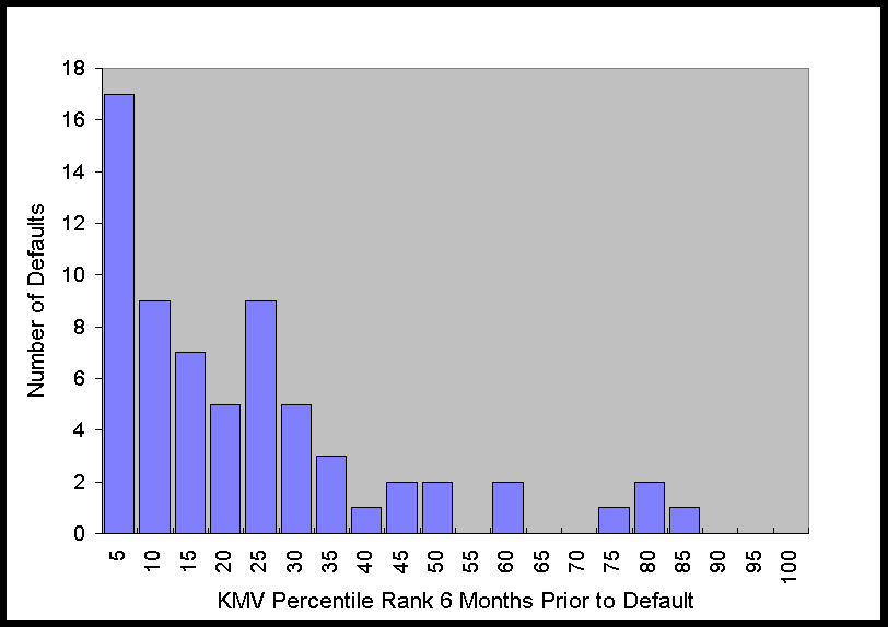
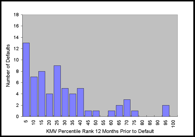
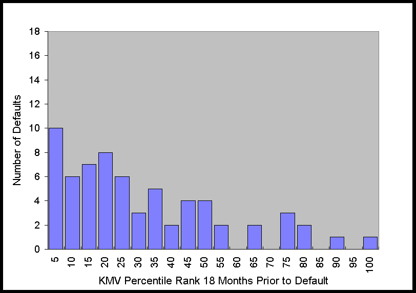
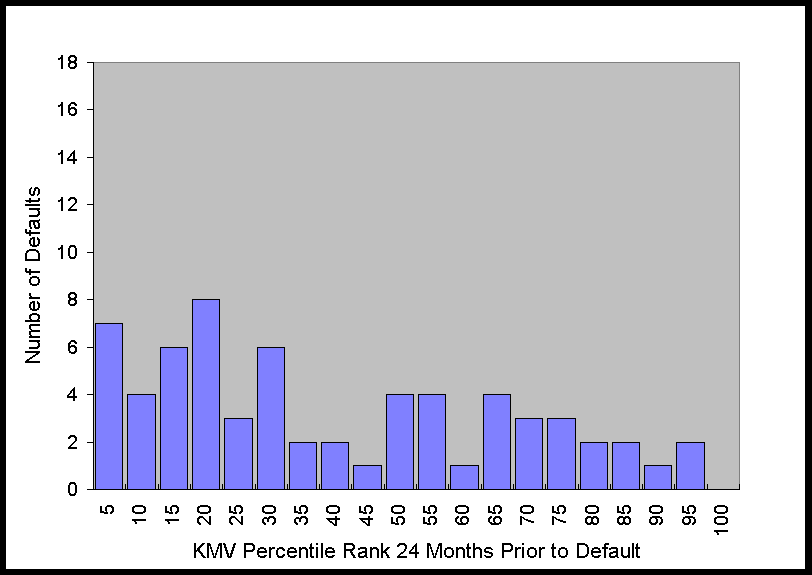
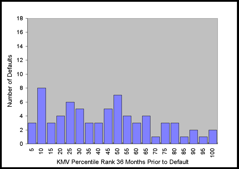
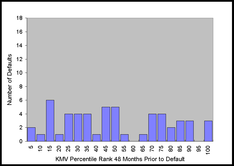
Figure 2. Distribution of KMV Percentiles of Defaulting Firms 6 to 48 Months Prior to Default

Copyright © 1998 by Miller Risk Advisors. All rights reserved.